Introduction
Going into this project I had a vision of somehow plotting my cycling routes on a realistic 3D map. Previously, I had mapped my routes on a 2D map to create a heat map but I felt like something was missing. It occured to me that I had the elevation data for all of these routes and it seemed likely that open source elevation data was available. Eventually I came across the Rayshader package and was blown away; it was exactly what I was looking for to create the 3D map. This article will go through how to create your own 3D mapped route. The source code is available on my github page
Steps
- 1. Load the route and extract the latitude and longitude
- 2. Select the map region
- 3. Get the elevation data
- 4. Get the overlay image
- 5. Plot the 3D map using rayshader
- 6. Plot the 3D route line
Load route and extract the latitude and longitude
If you are using a route recorded on a Garmin device, simply go to the activity you would like to plot in Garmin connect and download the gpx file for that activity. If you are using a different GPS device you will need to get the gpx file for the route. The file I chose is from a route I did last summer that went up Mt. Mitchell. Generally, the larger the elevations differences are the more interesting the 3D map will be. The gpx file format is actually an xml file so the XML package in R can be used to extract the necessary information. From there the data will be organized in a dataframe for easy access. The data from the gpx file may differ based on what devices you have connected to your GPS so your data my also include power or speed. If this is the case, adjust your dataframe accordingly.
		filename <- "route.gpx"
		gpx.raw <- xmlTreeParse(filename, useInternalNodes = TRUE)
		rootNode <- xmlRoot(gpx.raw)
		gpx.rawlist <- xmlToList(rootNode)$trk
		gpx.list <- unlist(gpx.rawlist[names(gpx.rawlist) == "trkseg"], recursive = FALSE)
		gpx <- do.call(rbind.fill, lapply(gpx.list, function(x) as.data.frame(t(unlist(x)), stringsAsFactors=F)))
		names(gpx) <- c("time","ele", "hr", "temp", "lat", "lon")

		# Convert column classes
		gpx[3:6] <- data.matrix(gpx[3:6])
		sapply(gpx[3:6], class)
		gpx[3:6] = as.numeric(unlist(gpx[3:6]))

		gpx$time <- sub("T", " ", gpx$time)
		gpx$time <- sub("\\+00:00","",gpx$time)
		gpx$time  <- as.POSIXlt(gpx$time)
		gpx$ele <- as.numeric(gpx$ele)

		gpx <- gpx[,c("time","hr","temp","lon","lat","ele")]
Select the map region
Once the data is loaded into the dataframe you will have access to the latitude and longitude values for that route. We will use the minimum and maximum for latitude and longitude to select the region for the 3D map.
		lat_min <- min(gpx$lat)
		lat_max <- max(gpx$lat)
		long_min <- min(gpx$lon)
		long_max <- max(gpx$lon)
Get the elevation data
The next step is to get the elevation data. Using the elevatr package, which pulls the data from AWS tiles makes this step straightforward. We will input the minimum and maximum for latitude and longitude and a coordinate reference system. The z factor goes from 0-14 and affects the resolution for the elevation data with 14 being the highest resolution. The next step is to get the dimensions of the raster. This will be important for overlaying an image of the DEM (digital elevation map). Rayshader requires a matrix input so the raster is converted to a matrix.
		ex.df <- data.frame(x= c( long_min, long_max),
                    y=c(lat_min,lat_max))
		prj_dd <- "+proj=longlat +ellps=WGS84 +datum=WGS84 +no_defs"
		elev_img <- get_elev_raster(ex.df, prj = prj_dd, z = 12, clip = "bbox")
		elev_tif <- raster::writeRaster(elev_img, "Images/elevation.tif",overwrite= TRUE)
		dim <- dim(elev_tif)
		elev_matrix <- matrix(
		  raster::extract(elev_img, raster::extent(elev_img), buffer = 1000),
		  nrow = ncol(elev_img), ncol = nrow(elev_img))
Get the overlay image
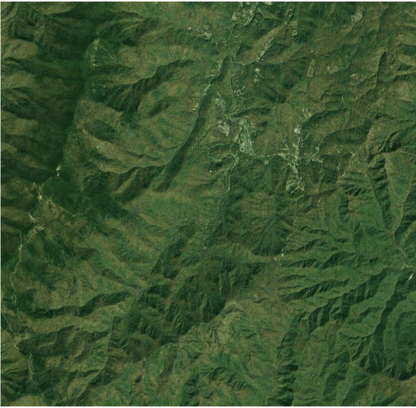
The clearest satellite image for the area I was interested in was from google maps. Obtaining the images from google maps can be a bit of a pain. I used the ggmap package to do this. Before you can use the get_googlemap() function you will have to register with google. That process is documented here . The next issue is that the google maps api doesn’t let you use a bounding box to obtain the area you want. Instead, it uses a center point and zoom to define the area. To get right bounding box, the center and zoom are set to return a raster that is larger than the desired bbox. The next step is to crop the raster to the desired coordinates and save the image as a png. For the region I selected the image was a bit dark when overlaid on the 3D map so I added filters and increased the contrast and brightness.
		long_cen <- (((long_max - long_min)/2) + long_min)
		lat_cen <- ((lat_max - lat_min)/2)+ lat_min
		mt_mit_map <- get_googlemap(center = c(lon= long_cen , lat = lat_cen), zoom = 12,
									maptype = "satellite", color = "color")

		# Plot overlay image and crop to the correct dimensions
		png("Images/overlay_image1.png", width=dim[2], height=dim[1], units= "px",type = "cairo-png")

		ggmap(mt_mit_map)+
			  scale_x_continuous(limits = c(long_min, long_max), expand = c(0, 0)) +
			  scale_y_continuous(limits = c(lat_min, lat_max), expand = c(0, 0))+
			  theme(axis.line = element_blank(),
					axis.text = element_blank(),
					axis.ticks = element_blank(),
					plot.margin = unit(c(0, 0, -1, -1), 'lines')) +
			  xlab('') +
			  ylab('')

		dev.off()
		# Edit Image
		image <- "Image/overlay_image.png"
		image <- image_read(image)
		green<- image_colorize(image=image,"#08c72e", opacity = 2 )
		yellow <- image_colorize(image=green,"#eaf518", opacity = 6 )
		contrast<- image_contrast(yellow, sharpen = 10)
		final <- image_modulate(contrast, brightness = 120)
		image_write(final, path= "Images/overlay_image.png")

		overlay_file <- "Images/overlay_image.png"
		overlay_img <- png::readPNG(overlay_file)
Plot the 3D map using Rayshader
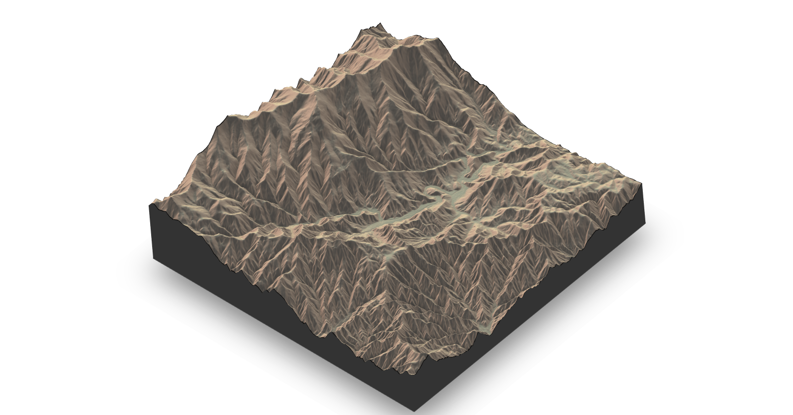
Below is the resulting 3D map without the overlay image. Once you run the code, you will be able to rotate the map in 3D. This map does not look very realistic since the region I mapped was located and the blue ridge mountains.
		 #Calculate rayshader layers
			ambmat <- ambient_shade(elev_matrix, zscale = 8)
			raymat <- ray_shade(elev_matrix, zscale = 8, lambert = TRUE)
			watermap <- detect_water(elev_matrix, zscale = 8)

		# Create the 3D Map
			zscale <- zscale
			rgl::clear3d()
			elev_matrix %>%
				  sphere_shade(texture = "imhof4") %>%
				  add_water(watermap, color = "imhof4") %>%
				  add_shadow(raymat, max_darken = 0.5) %>%
				  add_shadow(ambmat, max_darken = 0.5) %>%
				  plot_3d(elev_matrix,zscale =7)
Adding the overlay image in Rayshader is quite easy.
		#Calculate rayshader layers
			ambmat <- ambient_shade(elev_matrix, zscale = 8)
			raymat <- ray_shade(elev_matrix, zscale = 8, lambert = TRUE)
			watermap <- detect_water(elev_matrix, zscale = 8)
		# Create the 3D Map
			zscale <- 7
			rgl::clear3d()
			elev_matrix %>%
				  sphere_shade(texture = "imhof4") %>%
				  add_water(watermap, color = "imhof4") %>%
				  add_overlay(overlay_img, alphalayer = .9) %>%
				  add_shadow(raymat, max_darken = 0.5) %>%
				  add_shadow(ambmat, max_darken = 0.5) %>%
				  plot_3d(elev_matrix,zscale = zscale)
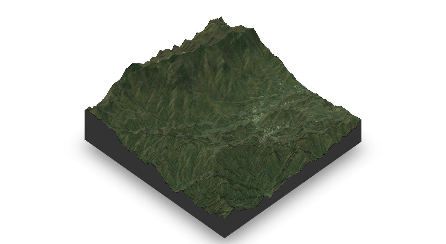
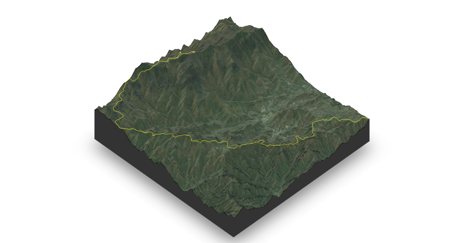
That looks pretty good. Next we’ll add the GPS route.
Plot the 3D route line
The rayshader package uses the rgl package to plot in 3D so the rgl package can be used to plot the route as well. We will use the rgl::lines3d() function. This function takes x, y , z arguments. X is the longitude, y is the latitude, z is the elevation. The map from rayshader is created using a raster matrix. This means that each cell has an elevation value and each cell represents a width and length value in the real world (eg. a cell may represent a 1m x 1m piece of land). So the latitude and longitude values from the route need to be converted to the correct cell in order to be plotted. This is done by subtracting the longitude minimum from each longitude value and dividing by the cell size in the longitude direction. The same is done for the latitude values. Then the elevation values are extracted from the elevation raster at the latitude/longitude coordinates on the route.
		# Convert lat and long to rayshader grid
		xmin <- elev_img@extent@xmin
		ymin <- elev_img@extent@ymin

		xmin_vec <- rep(xmin,length(gpx$lon))
		ymin_vec <- rep(ymin,length(gpx$lat))
		x <- (gpx$lon-xmin_vec)/ res(elev_img)[1]
		y <- (gpx$lat-ymin_vec)/ res(elev_img)[2]
		z <- extract(elev_img, gpx[,c(4,5)])


		# Plot the route in 3D
		rgl::lines3d(
			  x,
			  z/(zscale-.08),
			  -y,
			  color = "yellow",
			  add= TRUE
		)
Conclusion
That is it for this post. There is a lot more that can be done using the rayshader package. I hope you learned something useful!